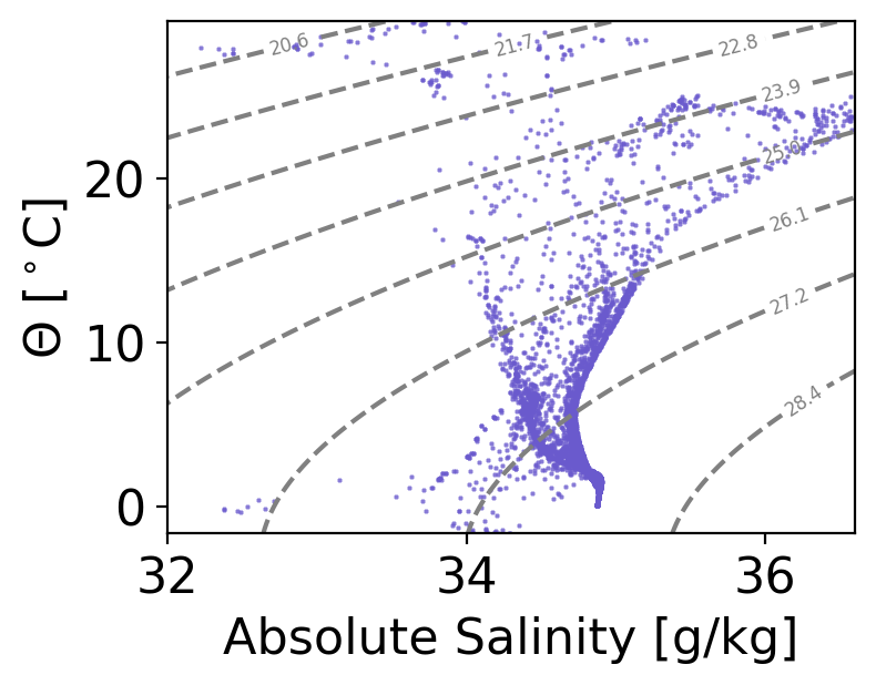
Explore Bottle File Data from CCHDO

In this notebook we will plot data from a bottle file, collected on a repeat hydrographic section part of the GO-SHIP repeat hydrographic program.

All hydrographic data part of this progam are publicly avaiable and are archived at CCHDO. The section analyzed here (P18) is a meridonal transect in the eastern Pacific roughly along the 103\(^o\)W meridian. Section data is available at https://cchdo.ucsd.edu/cruise/33RO20161119. The netCDF file for the bottle data can be downloaded here.

import xarray as xr
import pandas as pd
import numpy as np
import datetime
import matplotlib.pyplot as plt
import matplotlib.cm as cm
import cartopy.crs as ccrs
import gsw
%matplotlib inline

plt.rcParams["font.size"] = 16
plt.rcParams["figure.facecolor"] = 'white'
import warnings
warnings.filterwarnings('ignore')

datapath = './data/'

# Load netCDF file locally as xarray Dataset

dd = xr.load_dataset(datapath+'p18_btl.nc')
dd

<xarray.Dataset>
Dimensions:                            (N_LEVELS: 24, N_PROF: 213)
Coordinates:
    expocode                           (N_PROF) object '33RO20161119' ... '33...
    station                            (N_PROF) object '1' '2' ... '211' '212'
    cast                               (N_PROF) int32 3 2 1 1 1 1 ... 1 1 1 1 1
    sample                             (N_PROF, N_LEVELS) object '24' ... '1'
    time                               (N_PROF) datetime64[ns] 2016-11-24T14:...
    latitude                           (N_PROF) float64 22.69 22.87 ... -68.07
    longitude                          (N_PROF) float64 -110.0 -110.0 ... -95.0
    pressure                           (N_PROF, N_LEVELS) float64 3.1 ... 4.5...
Dimensions without coordinates: N_LEVELS, N_PROF
Data variables: (12/86)
    section_id                         (N_PROF) object 'P18' 'P18' ... 'P18'
    bottle_number                      (N_PROF, N_LEVELS) object '11122' ... ...
    bottle_number_qc                   (N_PROF, N_LEVELS) float32 2.0 ... 2.0
    btm_depth                          (N_PROF) float64 2.619e+03 ... 4.429e+03
    ctd_temperature                    (N_PROF, N_LEVELS) float64 27.88 ... 0...
    ctd_salinity                       (N_PROF, N_LEVELS) float64 34.53 ... 34.7
    ...                                 ...
    n2_argon_ratio_unstripped_error    (N_PROF, N_LEVELS) float64 nan ... nan
    d15n_n2                            (N_PROF, N_LEVELS) float64 nan ... nan
    d15n_n2_qc                         (N_PROF, N_LEVELS) float32 nan ... nan
    d15n_n2_error                      (N_PROF, N_LEVELS) float64 nan ... nan
    profile_type                       (N_PROF) object 'B' 'B' 'B' ... 'B' 'B'
    geometry_container                 float64 nan
Attributes:
    Conventions:               CF-1.8 CCHDO-1.0
    cchdo_software_version:    hydro 1.0.2.8
    cchdo_parameters_version:  params 2024.4.0
    comments:                  BOTTLE,20230606CCHSIOCBG\n Merged parameters: ...
    featureType:               profile

# List the variables in this bottle file
all_vars = [i for i in dd.data_vars] 
print(all_vars)

['section_id', 'bottle_number', 'bottle_number_qc', 'btm_depth', 'ctd_temperature', 'ctd_salinity', 'ctd_salinity_qc', 'bottle_salinity', 'bottle_salinity_qc', 'ctd_oxygen', 'ctd_oxygen_qc', 'oxygen', 'oxygen_qc', 'silicate', 'silicate_qc', 'nitrate', 'nitrate_qc', 'nitrite', 'nitrite_qc', 'phosphate', 'phosphate_qc', 'cfc_11', 'cfc_11_qc', 'cfc_12', 'cfc_12_qc', 'sulfur_hexifluoride', 'sulfur_hexifluoride_qc', 'total_carbon', 'total_carbon_qc', 'total_alkalinity', 'total_alkalinity_qc', 'ph_sws', 'ph_sws_qc', 'ph_temperature', 'dissolved_organic_carbon', 'dissolved_organic_carbon_qc', 'del_carbon_13_dic', 'del_carbon_13_dic_qc', 'del_carbon_14_dic', 'del_carbon_14_dic_qc', 'del_carbon_14_dic_error', 'particulate_organic_carbon', 'particulate_organic_carbon_qc', 'particulate_organic_nitrogen', 'particulate_organic_nitrogen_qc', 'total_dissolved_phosphorus', 'total_dissolved_phosphorus_qc', 'total_dissolved_nitrogen', 'total_dissolved_nitrogen_qc', 'carbon_tetrachloride', 'carbon_tetrachloride_qc', 'nitrous_oxide', 'nitrous_oxide_qc', 'nitrous_oxide_l_alt_1', 'nitrous_oxide_l_alt_1_qc', 'dissolved_organic_carbon_14', 'dissolved_organic_carbon_14_qc', 'dissolved_organic_carbon_14_error', 'dissolved_organic_carbon_13', 'dissolved_organic_carbon_13_qc', 'd15n_no3', 'd15n_no3_qc', 'd15n_no3_error', 'd15n_n2o', 'd15n_n2o_qc', 'd15n_alpha_n2o', 'd15n_alpha_n2o_qc', 'd15n_nitrite_nitrate', 'd15n_nitrite_nitrate_qc', 'd18o_nitrite_nitrate', 'd18o_nitrite_nitrate_qc', 'd18o_nitrate', 'd18o_nitrate_qc', 'd18o_nitrust_oxide', 'd18o_nitrust_oxide_qc', 'n2_argon_ratio', 'n2_argon_ratio_qc', 'n2_argon_ratio_error', 'n2_argon_ratio_unstripped', 'n2_argon_ratio_unstripped_qc', 'n2_argon_ratio_unstripped_error', 'd15n_n2', 'd15n_n2_qc', 'd15n_n2_error', 'profile_type', 'geometry_container']

exclude_vars = ['bottle_number']  # exclude these variables

# get a list of variables that we might be interested in-
# Filter remove one dimensional variables, QC flags and error variables

vars_of_interest = [i for i in all_vars if '_qc' not in i and '_error' not in i
                    and i not in exclude_vars 
                    and len(dd[i].dims)==2]
print(vars_of_interest)

['ctd_temperature', 'ctd_salinity', 'bottle_salinity', 'ctd_oxygen', 'oxygen', 'silicate', 'nitrate', 'nitrite', 'phosphate', 'cfc_11', 'cfc_12', 'sulfur_hexifluoride', 'total_carbon', 'total_alkalinity', 'ph_sws', 'ph_temperature', 'dissolved_organic_carbon', 'del_carbon_13_dic', 'del_carbon_14_dic', 'particulate_organic_carbon', 'particulate_organic_nitrogen', 'total_dissolved_phosphorus', 'total_dissolved_nitrogen', 'carbon_tetrachloride', 'nitrous_oxide', 'nitrous_oxide_l_alt_1', 'dissolved_organic_carbon_14', 'dissolved_organic_carbon_13', 'd15n_no3', 'd15n_n2o', 'd15n_alpha_n2o', 'd15n_nitrite_nitrate', 'd18o_nitrite_nitrate', 'd18o_nitrate', 'd18o_nitrust_oxide', 'n2_argon_ratio', 'n2_argon_ratio_unstripped', 'd15n_n2']

# Calculate Depth as a function of pressure, latitude
depth = gsw.z_from_p(dd.pressure,
                     dd.latitude,)

We can plot some of these variables of interest in a subplot together

1. Lets plot 16 variables in a 4x4 grid

2. Select a profile number profile_num to plot these 25 variables from

3. Select some plotting colors

4. Loop through these and plot

num_plots = 16  # number of variables to plot
profile_num = 190 # select profile number to plot 

# Choose the colormap
cmap = cm.get_cmap('Spectral')
# Get evenly spaced colors from the colormap
colors = [cmap(i) for i in np.linspace(0, 256, num_plots, dtype=int)]

num_rows = int(np.sqrt(num_plots))
num_cols = int(np.sqrt(num_plots))
fig, axs = plt.subplots(num_rows, num_cols, figsize=(10, 10),sharey=True)
# Loop through variables and plot in each subplot
for i, var in enumerate(vars_of_interest[:16]):
    # Calculate subplot index
    row = i // num_rows
    col = i % num_cols
    
    # Plot variable on the corresponding subplot
    axs[row, col].plot(dd[var][profile_num],depth[profile_num], 
                       label=var,linewidth='4',color=colors[i])
    axs[row, col].set_title(var)
    axs[row, col].set_ylabel('Depth [m]')

plt.tight_layout()  # Adjust layout
plt.show()  # Show the plot

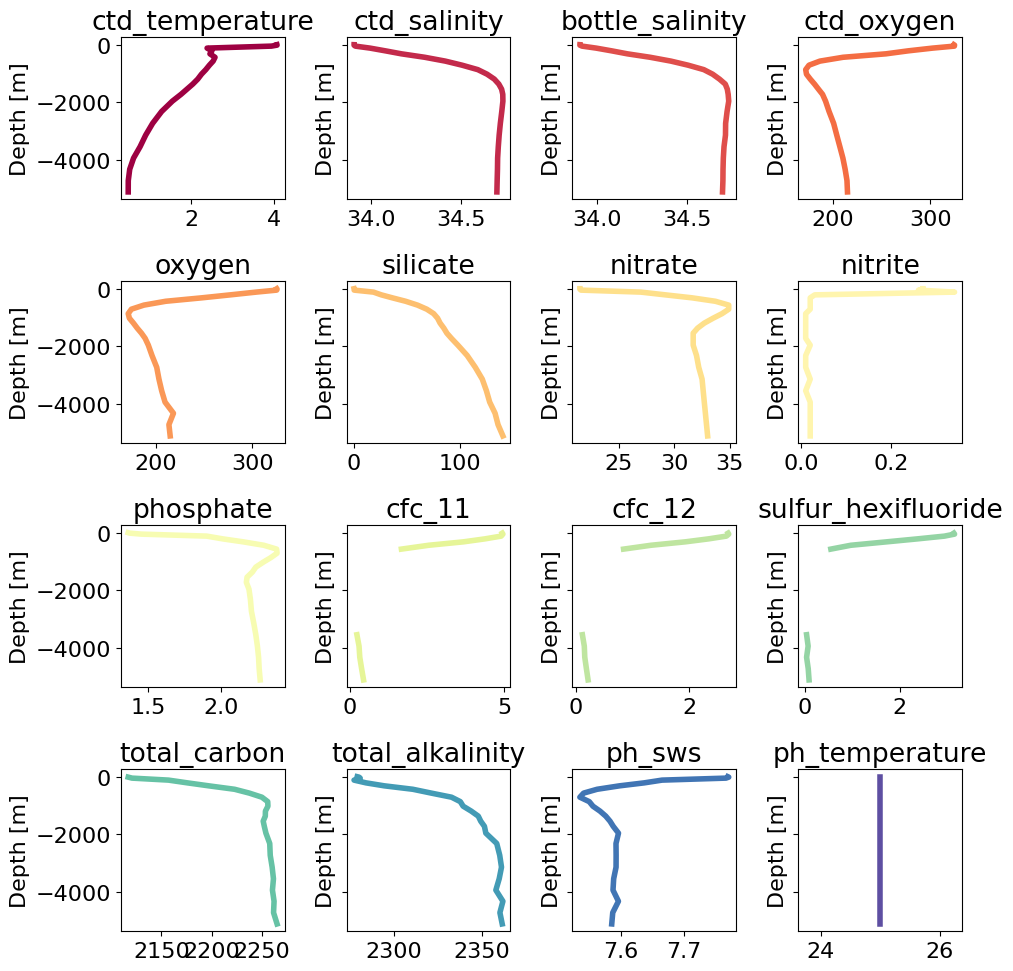
Next, we can calculate Absolute Salinity (SA) and Conservative Temperature (\(\Theta\)) and Potential Density (\(\sigma_0\))using the GSW Toolbox

dd['SA'] = gsw.SA_from_SP(dd.ctd_salinity, dd.pressure, dd.longitude, dd.latitude)
dd['CT'] = gsw.CT_from_t(dd.SA,dd.ctd_temperature, dd.pressure)
dd['sigma_0'] = gsw.sigma0(dd.SA,dd.CT)

Now we can plot a T-S diagram using this information for all profiles along the section.

We will also contour potential density, which is useful to identify water masses and water-mass transformation

plt.figure(figsize=(4,3),dpi=200)

# Create a grid of SA and CT values using meshgrid
SA_vals = np.linspace(dd.SA.min(), dd.SA.max(), 100)
CT_vals = np.linspace(dd.CT.min(), dd.CT.max(), 100)
SA_grid, CT_grid = np.meshgrid(SA_vals, CT_vals)

# Calculate potential density at each point on the grid
p_density = gsw.sigma0(SA_grid, CT_grid)  # Assuming reference pressure of 0 dbar
# Scatter plot of Absolute Salinity vs. Conservative Temperature
plt.plot(dd.SA, dd.CT, 
         color='slateblue',
         marker='+',
         markersize=1.2,
         alpha=0.8,
         linestyle='')

# Add potential density contours
density_levels = np.linspace(min(p_density.flatten()), max(p_density.flatten()), 10)  # Choose density levels
CS = plt.contour(SA_grid, CT_grid, p_density, 
                 levels=density_levels, 
                 colors='gray', 
                 linestyles='dashed')
plt.clabel(CS, inline=True, fontsize=6, fmt='%.1f')

# Label axes
plt.xlabel('Absolute Salinity [g/kg]')
plt.ylabel(r'$\Theta$ [$^\circ$C]')

# Set axis limit
plt.xlim(32,36.6)
plt.show()