Combine CTD and Bottle Data Files

In this notebook we will plot data from a bottle file, collected on a repeat hydrographic section part of the GO-SHIP repeat hydrographic program.

All hydrographic data part of this progam are publicly avaiable and are archived at CCHDO. The section analyzed here (P18) is a meridonal transect in the eastern Pacific roughly along the 103\(^o\)W meridian. Section CTD data is available at https://cchdo.ucsd.edu/cruise/33RO20161119. The netCDF file for the bottle data can be downloaded here.

import xarray as xr
import pandas as pd
import numpy as np
import datetime
import matplotlib.pyplot as plt
import matplotlib.cm as cm
import cartopy.crs as ccrs
import gsw
%matplotlib inline

plt.rcParams["font.size"] = 16
plt.rcParams["figure.facecolor"] = 'white'
import warnings
warnings.filterwarnings('ignore')

datapath = './data/'

# Load netCDF file for ctd and bottle files locally as xarray Dataset
ds_ctd = xr.load_dataset(datapath+'p18.nc')
ds_btl = xr.load_dataset(datapath+'p18_btl.nc')

First we can check if our CTD data is correctly loaded in

# Simple section plot of Pressure Levels vs along-section Profile
ds_ctd.ctd_salinity.T.plot(figsize=(20,5),yincrease=False,cmap='YlGnBu_r',vmax=35.,vmin=34.)
plt.show()

Notice that the Y-dimension of the plot above is in N_LEVELS which is just an index

Alternatively, it would be useful to plot this in terms of a physical quantity such as Pressure or Depth

# Linearly Interpolate Salinity onto regular pressure grid and store in a new variable
new_ds = ds_ctd.ctd_salinity.interp_like(ds_ctd.pressure, method='linear')
new_ds = new_ds.rename({'N_LEVELS':'PRESSURE'})  # rename dimension 

# Plot the new dataset variable like before (should be quite similar)
# Simple section plot of Pressure Levels vs along-section Profile
new_ds.T.plot(figsize=(20,5),yincrease=False,cmap='YlGnBu_r',vmax=35.,vmin=34.)
plt.show()

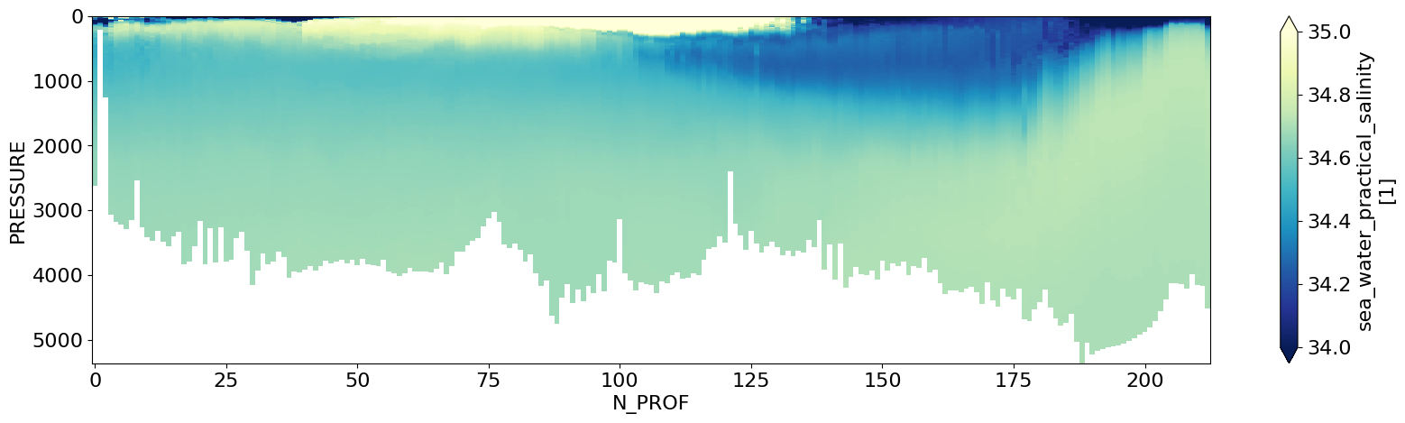
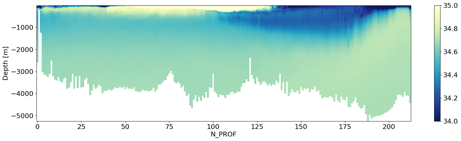
Instead of Pressure, we can also try plotting this versus depth.

Here is how-

# Calculate Depth as a function of pressure, latitude
depth = gsw.z_from_p(ds_ctd.pressure,
                     ds_ctd.latitude,)

# Next, we can store depth as a coordinate in our original dataset
ds_ctd = ds_ctd.assign_coords(depth=(('N_PROF', 'N_LEVELS'), depth.data))

# We can add some attributes to it
ds_ctd.depth.attrs = dict(whp_name='depth',whp_unit='meters',standard_name='depth')

ds_ctd.var() # display variables

<xarray.Dataset>
Dimensions:                     (N_LEVELS: 5364, N_PROF: 213)
Coordinates:
    expocode                    (N_PROF) object '33RO20161119' ... '33RO20161...
    station                     (N_PROF) object '1' '2' '3' ... '211' '212'
    cast                        (N_PROF) int32 3 2 1 1 1 1 1 1 ... 2 1 1 1 1 1 1
    sample                      (N_PROF, N_LEVELS) object '3.0' '4.0' ... '' ''
    time                        (N_PROF) datetime64[ns] 2016-11-24T14:17:00 ....
    latitude                    (N_PROF) float64 22.69 22.87 ... -70.0 -68.07
    longitude                   (N_PROF) float64 -110.0 -110.0 ... -100.2 -95.0
    pressure                    (N_PROF, N_LEVELS) float64 3.0 4.0 ... nan nan
    depth                       (N_PROF, N_LEVELS) float64 -2.981 -3.975 ... nan
Dimensions without coordinates: N_LEVELS, N_PROF
Data variables: (12/16)
    section_id                  (N_PROF) object 'P18' 'P18' ... 'P18' 'P18'
    btm_depth                   (N_PROF) float64 2.625e+03 ... 4.435e+03
    pressure_qc                 (N_PROF, N_LEVELS) float32 2.0 2.0 ... nan nan
    ctd_temperature             (N_PROF, N_LEVELS) float64 27.92 27.92 ... nan
    ctd_temperature_qc          (N_PROF, N_LEVELS) float32 3.0 3.0 ... nan nan
    ctd_salinity                (N_PROF, N_LEVELS) float64 34.53 34.53 ... nan
    ...                          ...
    ctd_beamcp                  (N_PROF, N_LEVELS) float64 nan 0.0479 ... nan
    ctd_beamcp_qc               (N_PROF, N_LEVELS) float32 nan 2.0 ... nan nan
    ctd_beta700_raw             (N_PROF, N_LEVELS) float64 0.076 0.076 ... nan
    ctd_number_of_observations  (N_PROF, N_LEVELS) float64 19.0 36.0 ... nan nan
    profile_type                (N_PROF) object 'C' 'C' 'C' 'C' ... 'C' 'C' 'C'
    geometry_container          float64 nan
Attributes:
    Conventions:               CF-1.8 CCHDO-1.0
    cchdo_software_version:    hydro 1.0.2.3
    cchdo_parameters_version:  params 0.1.21
    comments:                  CTD,20200213CCHSIO\n Parameters removed from E...
    featureType:               profile

# Plot dataset
plt.figure(figsize=(20,5))
plt.pcolor(ds_ctd.N_PROF,ds_ctd.depth[188,:],ds_ctd.ctd_salinity.T,cmap='YlGnBu_r',
           vmax=35.,vmin=34.)
plt.xlabel('N_PROF')
plt.ylabel('Depth [m]')
plt.colorbar()
plt.show()

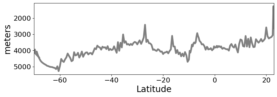
Next we can take a look at the bathymetry of this section

It can be useful to plot the maximum depth and which CTD station it corresponds to.

# Plot bottom bathymetry 
ds_ctd['btm_depth'].plot(figsize=(10,3),
                     yincrease=False,
                     x='latitude',
                     color='gray',
                     linewidth=4,
                     xlim=(-70,23),
                     )
plt.ylabel('meters',fontsize=20)
plt.xlabel('Latitude',fontsize=20)
plt.show()

# We can find the CTD station with the maximum bottom depth
STA_MAX_DEPTH = ds_ctd['btm_depth'].argmax()
print(STA_MAX_DEPTH.values)

188

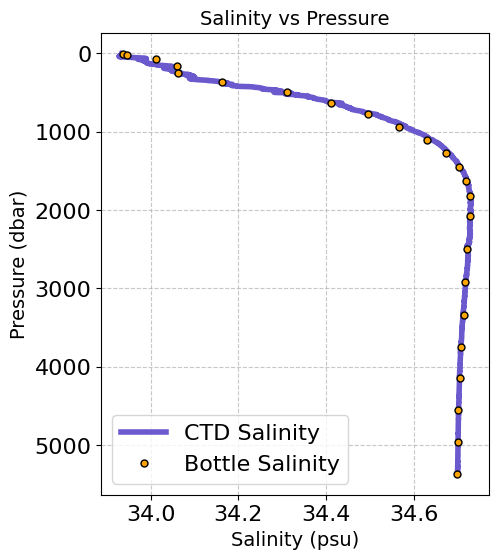
Now we can look at some corresponding Bottle and CTD data from this Station

# Create figure
plt.figure(figsize=(5, 6),dpi=100)

# Plot salinity data
plt.plot(ds_ctd.ctd_salinity[STA_MAX_DEPTH, :], ds_ctd.pressure[STA_MAX_DEPTH, :], 
         label='CTD Salinity', color='slateblue', linewidth=4,)

# Plot bottle salinity data
plt.plot(ds_btl.bottle_salinity[STA_MAX_DEPTH, :], ds_btl.pressure[STA_MAX_DEPTH, :], 
         'o', label='Bottle Salinity', color='orange', markersize=5, markeredgecolor='black')

# Invert pressure axis
plt.gca().invert_yaxis()

# Adding titles and labels
plt.title('Salinity vs Pressure', fontsize=14)
plt.xlabel('Salinity (psu)', fontsize=14)
plt.ylabel('Pressure (dbar)', fontsize=14)

plt.legend()
# Add grid
plt.grid(True, linestyle='--', alpha=0.7)

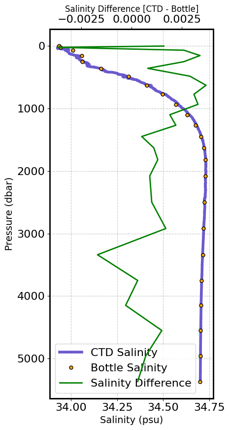
It is also useful sometimes to look at the CTD vs Bottle Mismatch

# Create figure
fig, ax1 = plt.subplots(figsize=(5, 9), dpi=100)

# Plot salinity data with labels on ax1 using the specified profile number
line_ctd, = ax1.plot(ds_ctd.ctd_salinity[STA_MAX_DEPTH, :], ds_ctd.pressure[STA_MAX_DEPTH, :], 
                     label='CTD Salinity', color='slateblue', linewidth=4)

# Plot bottle salinity data with labels on ax1 using the specified profile number
line_bottle, = ax1.plot(ds_btl.bottle_salinity[STA_MAX_DEPTH, :], ds_btl.pressure[STA_MAX_DEPTH, :], 
                        'o', label='Bottle Salinity', color='orange', markersize=5, markeredgecolor='black')

# Invert pressure axis
ax1.invert_yaxis()

# Set labels for the axes on ax1
ax1.set_xlabel('Salinity (psu)', fontsize=14)
ax1.set_ylabel('Pressure (dbar)', fontsize=14)

# Add grid
ax1.grid(True, linestyle='--', alpha=0.7)

# Create a second x-axis on the top using ax2
ax2 = ax1.twiny()

# Calculate the difference between CTD and Bottle salinity using the specified profile number
salinity_difference = ds_btl.ctd_salinity[STA_MAX_DEPTH, :] - ds_btl.bottle_salinity[STA_MAX_DEPTH, :]

# Plot the difference on the second x-axis
line_difference, = ax2.plot(salinity_difference, ds_btl.pressure[STA_MAX_DEPTH, :], 
                             color='green', linewidth=2, label='Salinity Difference')

# Set label for the second x-axis
ax2.set_xlabel('Salinity Difference [CTD - Bottle]', fontsize=12)

# Combine legends from both axes
lines = [line_ctd, line_bottle, line_difference]  # List of handles for the legend
labels = [line.get_label() for line in lines]  # Get the labels from the handles
ax1.legend(lines, labels, loc='lower left')  # Create a single legend

# Make axis splines bold
ax1.spines['top'].set_linewidth(2)   # Top spine for ax1
ax1.spines['bottom'].set_linewidth(2) # Bottom spine for ax1
ax1.spines['left'].set_linewidth(2)   # Left spine for ax1
ax1.spines['right'].set_linewidth(2)  # Right spine for ax1
ax2.spines['top'].set_linewidth(2)     # Top spine for ax2
ax2.spines['bottom'].set_linewidth(2)  # Bottom spine for ax2

# Display the plot
plt.tight_layout()
plt.show()