Explore Repeat Hydrography Data from CCHDO

In this example notebook we will explore data collected on a repeat hydrographic section part of the GO-SHIP repeat hydrographic program.

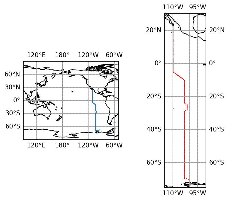
All hydrographic data part of this progam are publicly avaiable and are archived at CCHDO. The section analyzed here (P18) is a meridonal transect in the eastern Pacific roughly along the 103\(^o\)W meridian. Section data is available at https://cchdo.ucsd.edu/cruise/33RO20161119. The netCDF file for the CTD data can be downloaded here.

import xarray as xr
import pandas as pd
import numpy as np
import datetime
import matplotlib.pyplot as plt
import cartopy.crs as ccrs
import gsw
%matplotlib inline

plt.rcParams["font.size"] = 16
plt.rcParams["figure.facecolor"] = 'white'
import warnings
warnings.filterwarnings('ignore')

# local path to data
datapath = './data/'

# Load netCDF file locally as xarray Dataset

ds = xr.load_dataset(datapath+'p18.nc')
ds

<xarray.Dataset>
Dimensions:                     (N_LEVELS: 5364, N_PROF: 213)
Coordinates:
    expocode                    (N_PROF) object '33RO20161119' ... '33RO20161...
    station                     (N_PROF) object '1' '2' '3' ... '211' '212'
    cast                        (N_PROF) int32 3 2 1 1 1 1 1 1 ... 2 1 1 1 1 1 1
    sample                      (N_PROF, N_LEVELS) object '3.0' '4.0' ... '' ''
    time                        (N_PROF) datetime64[ns] 2016-11-24T14:17:00 ....
    latitude                    (N_PROF) float64 22.69 22.87 ... -70.0 -68.07
    longitude                   (N_PROF) float64 -110.0 -110.0 ... -100.2 -95.0
    pressure                    (N_PROF, N_LEVELS) float64 3.0 4.0 ... nan nan
Dimensions without coordinates: N_LEVELS, N_PROF
Data variables: (12/16)
    section_id                  (N_PROF) object 'P18' 'P18' ... 'P18' 'P18'
    btm_depth                   (N_PROF) float64 2.625e+03 ... 4.435e+03
    pressure_qc                 (N_PROF, N_LEVELS) float32 2.0 2.0 ... nan nan
    ctd_temperature             (N_PROF, N_LEVELS) float64 27.92 27.92 ... nan
    ctd_temperature_qc          (N_PROF, N_LEVELS) float32 3.0 3.0 ... nan nan
    ctd_salinity                (N_PROF, N_LEVELS) float64 34.53 34.53 ... nan
    ...                          ...
    ctd_beamcp                  (N_PROF, N_LEVELS) float64 nan 0.0479 ... nan
    ctd_beamcp_qc               (N_PROF, N_LEVELS) float32 nan 2.0 ... nan nan
    ctd_beta700_raw             (N_PROF, N_LEVELS) float64 0.076 0.076 ... nan
    ctd_number_of_observations  (N_PROF, N_LEVELS) float64 19.0 36.0 ... nan nan
    profile_type                (N_PROF) object 'C' 'C' 'C' 'C' ... 'C' 'C' 'C'
    geometry_container          float64 nan
Attributes:
    Conventions:               CF-1.8 CCHDO-1.0
    cchdo_software_version:    hydro 1.0.2.3
    cchdo_parameters_version:  params 0.1.21
    comments:                  CTD,20200213CCHSIO\n Parameters removed from E...
    featureType:               profile

# list all variables in the dataset
all_vars = [i for i in ds.data_vars] 
all_vars

['section_id',
 'btm_depth',
 'pressure_qc',
 'ctd_temperature',
 'ctd_temperature_qc',
 'ctd_salinity',
 'ctd_salinity_qc',
 'ctd_oxygen',
 'ctd_oxygen_qc',
 'ctd_fluor_raw',
 'ctd_beamcp',
 'ctd_beamcp_qc',
 'ctd_beta700_raw',
 'ctd_number_of_observations',
 'profile_type',
 'geometry_container']

# Plot this hydrogrphic line on a MAP, and show station locations 

projection = ccrs.PlateCarree(central_longitude=180.0)

fig = plt.figure(figsize=(6,5),dpi=150)
ax1 = fig.add_subplot(121, projection=projection)
ax1.set_extent((90,310, -90, 90))
ax1.coastlines()
ax1.gridlines()
ax1.plot(ds.longitude,ds.latitude,transform = ccrs.PlateCarree())

gl1 = ax1.gridlines(
    draw_labels=True, linewidth=1, color='gray', alpha=0.4, linestyle='--',)
# Adjust fontsize for tick labels
gl1.xlabel_style = {'size': 10}
gl1.ylabel_style = {'size': 10}

# add subplot for station locations
ax2 = fig.add_subplot(122, projection=projection)
ax2.set_extent((-115,-90, -75, 30))
ax2.coastlines()
ax2.gridlines()
ax2.scatter(ds.longitude,ds.latitude,transform = ccrs.PlateCarree(),
            marker='.',s=1,
            color='r')

gl2 = ax2.gridlines(
    draw_labels=True, linewidth=1, color='gray', alpha=0.4, linestyle='--',)
# Adjust fontsize for tick labels
gl2.xlabel_style = {'size': 10}
gl2.ylabel_style = {'size': 10}

plt.show()

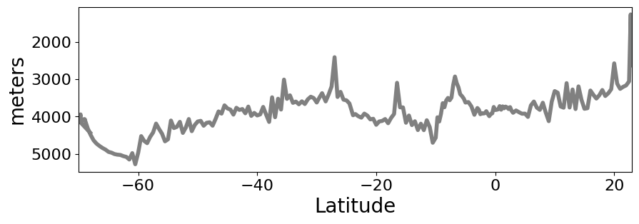
# Plot bottom bathymetry 
ds['btm_depth'].plot(figsize=(10,3),
                     yincrease=False,
                     x='latitude',
                     color='gray',
                     linewidth=4,
                     xlim=(-70,23),
                     )
plt.ylabel('meters',fontsize=20)
plt.xlabel('Latitude',fontsize=20)
plt.show()

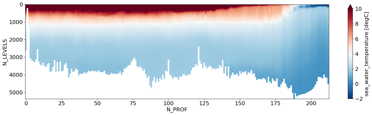
# Using xarray's plot wrapper, simple plot of Pressure Levels vs along-section Profile
ds.ctd_temperature.T.plot(figsize=(20,5),yincrease=False,cmap='RdBu_r',vmax=10,vmin=-2)
plt.show()

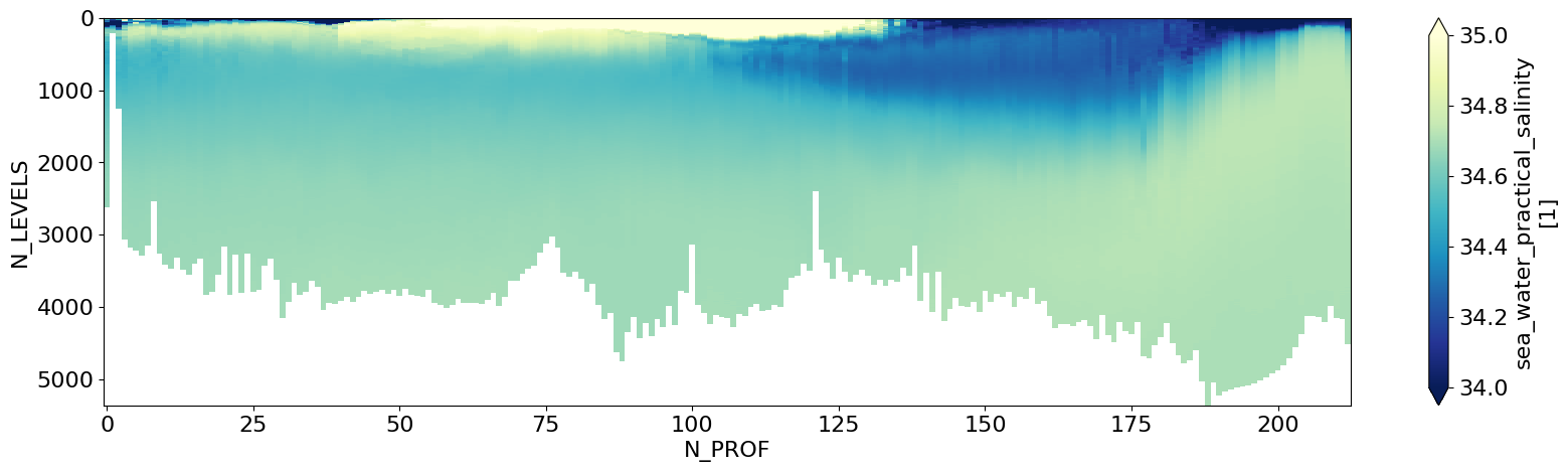
# Using xarray's plot wrapper, simple plot of Pressure Levels vs along-section Profile
ds.ctd_salinity.T.plot(figsize=(20,5),yincrease=False,cmap='YlGnBu_r',vmax=35.,vmin=34.)
plt.show()

Get some variables of interest in the dataset

exclude_vars = ['bottle_number']  # exclude these variables

# get a list of variables that we might be interested in-
# Filter remove one dimensional variables, QC flags and error variables

vars_of_interest = [i for i in all_vars if '_qc' not in i and '_error' not in i
                    and i not in exclude_vars 
                    and len(ds[i].dims)==2]
print(vars_of_interest)

['ctd_temperature', 'ctd_salinity', 'ctd_oxygen', 'ctd_fluor_raw', 'ctd_beamcp', 'ctd_beta700_raw', 'ctd_number_of_observations']

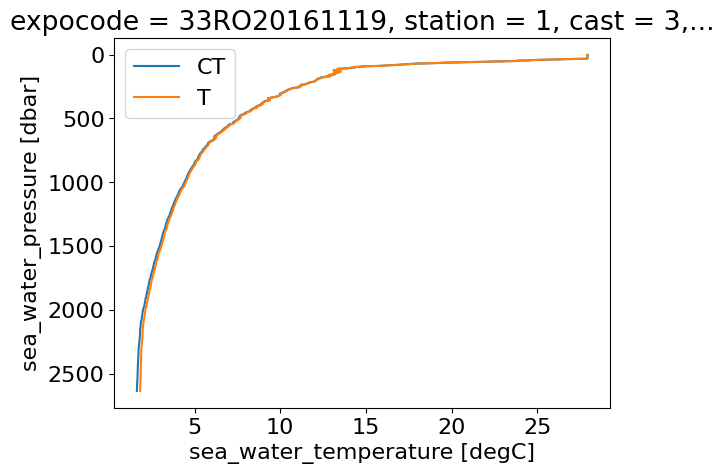
Next, we can calculate Absolute Salinity (SA) and Conservative Temperature (\(\Theta\)) and Potential Density (\(\sigma_0\))using the GSW Toolbox

ds['SA'] = gsw.SA_from_SP(ds.ctd_salinity, ds.pressure, ds.longitude, ds.latitude)
ds['CT'] = gsw.CT_from_t(ds.SA,ds.ctd_temperature, ds.pressure)
ds['sigma_0'] = gsw.sigma0(ds.SA,ds.CT)

# Plot CTD Temperature and Conservative Temperature vs Pressure Level for the first profile (index 0)
ds.CT.T[:,0].plot(y='pressure',yincrease=False,label='CT')
ds.ctd_temperature.T[:,0].plot(y='pressure',yincrease=False,label='T')
plt.legend()
plt.show()

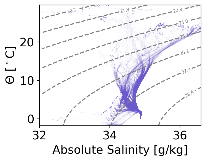
Now we can plot a T-S diagram using this information for all profiles along the section.

We will also contour potential density, which is useful to identify water masses and water-mass transformation

plt.figure(figsize=(4,3),dpi=200)

# Create a grid of SA and CT values using meshgrid
SA_vals = np.linspace(ds.SA.min(), ds.SA.max(), 100)
CT_vals = np.linspace(ds.CT.min(), ds.CT.max(), 100)
SA_grid, CT_grid = np.meshgrid(SA_vals, CT_vals)

# Calculate potential density at each point on the grid
p_density = gsw.sigma0(SA_grid, CT_grid)  # Assuming reference pressure of 0 dbar
# Scatter plot of Absolute Salinity vs. Conservative Temperature
plt.plot(ds.SA, ds.CT, 
         color='slateblue',
         marker='.',
         markersize=.1,
         alpha=0.2,
         linestyle='')

# Add potential density contours
density_levels = np.linspace(min(p_density.flatten()), max(p_density.flatten()), 10)  # Choose density levels
CS = plt.contour(SA_grid, CT_grid, p_density, 
                 levels=density_levels, 
                 colors='gray', 
                 linestyles='dashed')
plt.clabel(CS, inline=True, fontsize=6, fmt='%.1f')

# Label axes
plt.xlabel('Absolute Salinity [g/kg]')
plt.ylabel(r'$\Theta$ [$^\circ$C]')

# Set axis limit
plt.xlim(32,36.6)
plt.show()